Optimizing Iceberg MERGE Statements
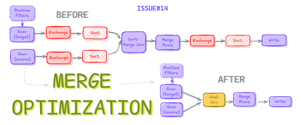
If you are using Apache Iceberg Tables and data is being shuffled, you might be doing something wrong!
You might think that's a very contradictory statement, and the safer way to say this can be with "It depends." – that's what I felt when I heard it for the first time. But if you stick to the end of this post, you will either figure out what you are doing wrong or learn something new.

TenorAlrighty, then, let's get into it.
We will take a very simple example for easier understanding and implement a MERGE statement and will further improve on it.
Setting up an Example
Let's assume we have a department data of an organization that has details of employee currently working in which department for a particular year.
So just 3 columns and one technical column:
id– Employee Id of an employeebusiness_vertical– Name of the Departmentyear– Year of workingis_updated– represents if employee has changed department
All this data will be stored in a Target Table.
In case employees are moved around different verticals, the business_vertical across their name also needs updation. All such employees data is sent into a different table, we will call this Staged Table
Initializing SparkSession with Iceberg
from pyspark.sql import SparkSession
from pyspark.sql.functions import rand, lit, array, rand, when, col

# Creating Spark Session
# Spark 3.5 with Iceberg 1.5.0

DW_PATH='/iceberg/spark/warehouse'
spark = SparkSession.builder \
    .master("local[4]") \
    .appName("iceberg-poc") \
    .config('spark.jars.packages', 'org.apache.iceberg:iceberg-spark-runtime-3.5_2.12:1.5.0')\
    .config('spark.sql.extensions','org.apache.iceberg.spark.extensions.IcebergSparkSessionExtensions')\
    .config('spark.sql.catalog.local','org.apache.iceberg.spark.SparkCatalog') \
    .config('spark.sql.catalog.local.type','hadoop') \
    .config('spark.sql.catalog.local.warehouse',DW_PATH) \
    .getOrCreate()
SparkSession Initialization
Generating and Populating Data into Table
We will be generating data for 3 years 2023 to 2025, along with id and business_vertical.
t1 = spark.range(30000).withColumn("year",
                                when(col("id") <= 10000, lit(2023))\
                                .when(col("id").between(10001, 15000), lit(2024))\
                                .otherwise(lit(2025))
                                )
t1 = t1.withColumn("business_vertical", array(
        lit("Retail"),
        lit("SME"),
        lit("Cor"),
        lit("Analytics")
        ).getItem((rand()*4).cast("int")))\
        .withColumn("is_updated", lit(False))
Data Generation
We will create a Merge-On-Read Table here to perform faster updates. You can read a detailed newsletter mentioned below if you are unsure about MOR.

Optimizing Row-level Updates
# Creating a table to store employee's business vertical info
TGT_TBL = "local.db.emp_bv_details"

t1.coalesce(1).writeTo(TGT_TBL).partitionedBy('year').using('iceberg')\
    .tableProperty('format-version','2')\
    .tableProperty('write.delete.mode','merge-on-read')\
    .tableProperty('write.update.mode','merge-on-read')\
    .tableProperty('write.merge.mode','merge-on-read')\
    .create()
Creating a Merge-On-Read Table: emp_bv_details
Updated Employee's Business Vertical Data
Let's assume 3000 employees have changed their departments to Sales in 2025.
# New department created called Sales and 3000 employees switched in 2025
updated_records = spark.range(15000, 18001).withColumn("year", lit(2025)).withColumn("business_vertical", lit("Sales"))

STG_TBL = "local.db.emp_bv_updates"

updated_records.coalesce(1).writeTo(STG_TBL).partitionedBy('year').using('iceberg')\
    .tableProperty('format-version','2')\
    .create()
Creating STAGE TABLE with employee update records
Merge Staging Data into Target Table
Now as we have all the data ready, let's merge this staging data with the data present in target table.
spark.sql(f"""
  MERGE INTO {TGT_TBL} as tgt
  USING (Select *, False as is_updated from {STG_TBL}) as src
  ON tgt.id = src.id
  WHEN MATCHED AND src.business_vertical <> tgt.business_vertical AND tgt.year = src.year THEN
      UPDATE SET tgt.is_updated = True, tgt.business_vertical = src.business_vertical
  WHEN NOT MATCHED THEN
      INSERT *
""")
MERGE statement to merge Staging Data into Target Table
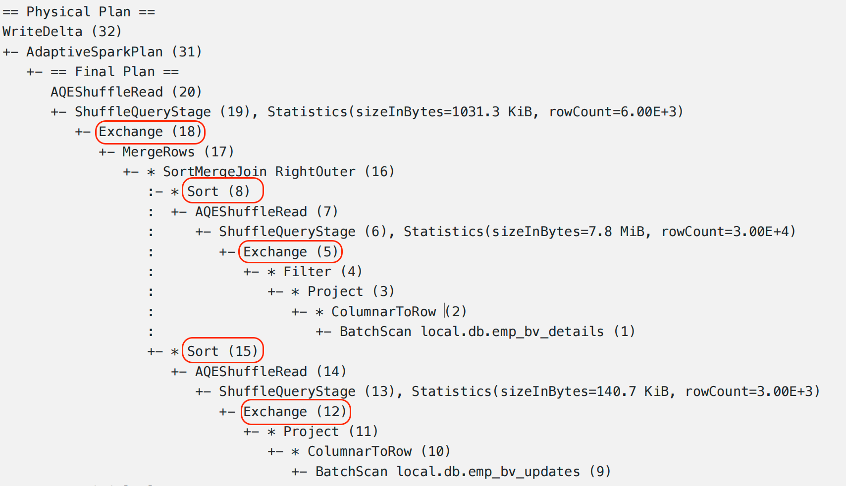
Merge Query Physical Plan. Expensive Operations are highlighted in RED.Merge Execution Plan
To understand what's happening under the hood of the MERGE statement, let's look into 3 sections of the Merge Execution Plan and the expensive parts within them.

redRead
- Scanning the source and target tables with the applied runtime filters.
- Expensive Operations: Scans without pushdown filters get unnecessary data into the memory.
Merge Rows
- Joining both the tables to compute the new state of the table by applying
WHEN MATCHEDandWHEN NOT MATCHEDclauses together to merge the records and create a new state of records - Expensive Operations: Shuffling and Sorting due to the Sort-Merge Join.
Write
- After merging the records, it's time to write them back into the target table.
- Expensive Operations: Pre-shuffling data before writing to align with the table partitioning scheme. (Optional) Pre-sorting of data before writing in case table has sort keys defined.
Exchange, a.k.a. Shuffling operations, will dominate the runtime of the MERGE Operation and will be, by far, the most expensive part of it.
Now that you know all the Expensive parts in all the sections, let's look into the Optimization techniques we can use to avoid or reduce these expensive operations.
Optimizing MERGE Statement
In this section we will be looking into the previous Merge Statement, identify the potential areas to improve it's performance.
Push Down Filters
This is a very common thing to miss out on while writing a MERGE Statement.
I mentioned missing out because you might still be using the required filter condition, but it might not get pushed down while reading from the table.
Let's take a look at previous MERGE Statement Scan Filters:
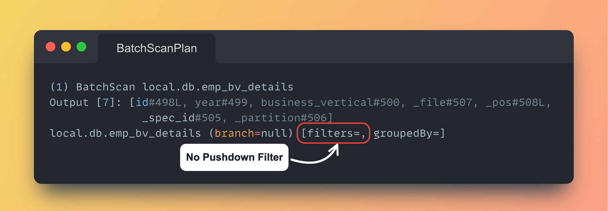
Pushdown FiltersTo push-down any filters it needs to be present in the ON clause of MERGE statement. Any filters present at WHEN MATCHED or WHEN NOT MATCHED are NOT pushed down.
-- Adding filter condition that will be pushed down
MERGE INTO TARGET_TABLE tgt
USING STAGE_TABLE stg
ON tgt.id = stg.id
  AND tgt.year = 2025 -- All filters in ON Clause are pushed down.
WHEN MATCHED ...
WHEN NOT MATCHED ...
ON Clause filters that will be pushed down

MERGE Plan after applying filters in ON ClauseSort-Merge Joins to Hash Joins (if possible)
Spark prefers Sort Merge Join by default because it's more scalable than Hash Join.
This behavior is controlled by Spark SQL Configuration spark.sql.join.preferSortMergeJoin which is set to true by default.
To overwrite this behavior, set spark.sql.join.preferSortMergeJoin to false. In cases where the build side is small enough to build a Hash Map, a Shuffle Hash Join will be preferred over Sort-Merge Join.
spark.conf.set("spark.sql.join.preferSortMergeJoin", "false")Setting preferSortMergeJoin to False
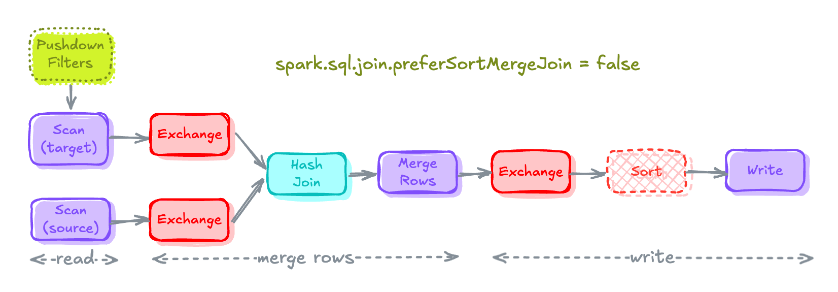
MERGE Execution Plan after preferSortMergeJoin is set to FalseIf you will notice the Sort that were caused by Sort Merge Join are eliminated.
Spark Fanout Writers
Local sorting happening before writing data can be avoided by enabling spark fan-out writers for the table.
This local sort is fairly cheaper in batch workloads compared to streaming workloads where it adds additional latency and can be avoided by using Fanout Writers.
# Setting Table Property to enable fanout-writers
spark.sql(f"""ALTER TABLE {TGT_TBL} SET TBLPROPERTIES (
    'write.spark.fanout.enabled'='true'
)""")
Enabling fanout Writers
Fanout writer opens the files per partition value and doesn't close these files till the write task finishes.
hadoop catalog but seems to work with the AWS glue catalog.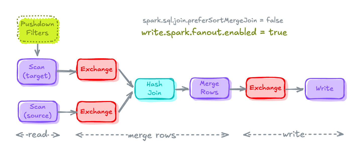
MERGE Execution Plan after fanout writers are enabledIceberg Distribution Modes
Distribution modes in Iceberg decides "How data is being distributed by IcebergWriter before it's being written into the Iceberg Table."
Iceberg provides 3 distribution modes:
None– Doesn't request for any shuffle or sort to be performed by Spark before writing data. Least expensive of all.hash– Requests data to be shuffled using hash based exchange by Spark before writing.range– Requests that Spark perform a range based exchange to shuffle the data before writing. Most expensive of all.
The Exchange node (Pre-shuffling before Write) present in write section of Merge Plan before writing data into table is because of the default distribution mode, i.e. hash.
This Exchange node can simply be eliminated by changing the distribution mode to None. This will accelerate the write process, BUT might end up in creating lots of small files.
# Setting Distribution mode in SparkSession.
# This overwrites the Distribution mode mentioned in TBLPROPERTIES
spark.conf.set("spark.sql.iceberg.distribution-mode", "None")
Setting Distribution-Mode as None in SparkSession
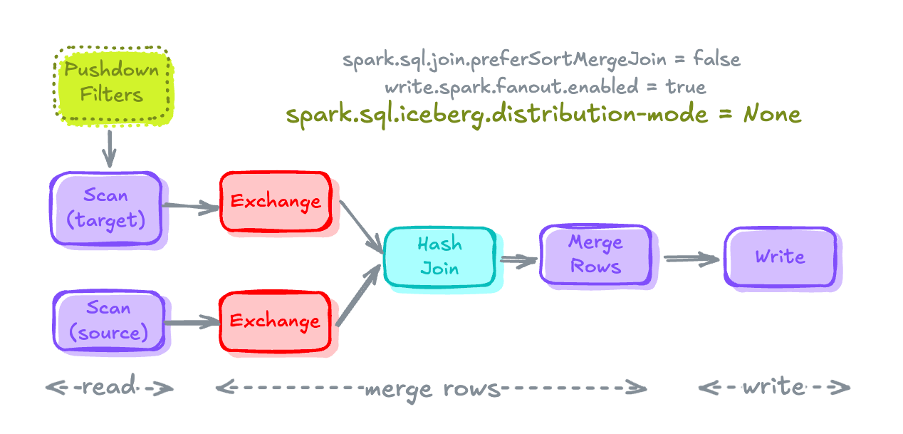
MERGE Execution Plan after Distribution Mode is set to NoneTrade-offs/Balancing between Write and Read Performance
Eliminating Exchange before writing into Table is a trade-off decision between Write Performance and Read Performance.Using None as a distribution mode can amplify the Write Performance but might degrade the Read Performance because of the creation of many small files.
Read Performance degradation can even be worse when you use MOR tables because while reading, the query engine will have to read many small files and the extra work it has to do to combine the records from the Delete file.
I mentioned balancing here because if you need both Write and Read performance, mitigating degradation in Read Performance requires frequent Compaction runs.
Does this mean we should never use None Distribution Mode?
You can still use None Distribution Mode, if you are:
- Writing data only in one partition, like in this case
year=2025. - Running Compaction frequently – To mitigate Read Performance Degradation, frequent Compaction runs is required.
- Write Performance is more important.
Main idea for this much details is to know what you are doing when you are making this decision.
Note: I am not covering how to mitigate the small file problem in this post as that is entirely a separate problem in itself.
Enabling Storage Partitioned Join
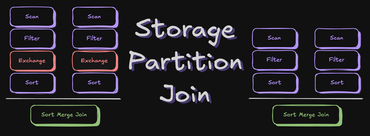
Storage Partitioned Join (SPJ) is a Join Optimization Technique that helps you avoid the expensive Shuffles while performing the joins.
You can read all about it 👇

Deep Dive into Storage Partitioned Join
To enable SPJ, there are 2 main things needs to be done:
Setting up Configurations for SPJ
# Enabling SPJ
spark.conf.set('spark.sql.sources.v2.bucketing.enabled','true')
spark.conf.set('spark.sql.sources.v2.bucketing.pushPartValues.enabled','true')
spark.conf.set('spark.sql.iceberg.planning.preserve-data-grouping','true')
spark.conf.set('spark.sql.requireAllClusterKeysForCoPartition','false')
spark.conf.set('spark.sql.sources.v2.bucketing.partiallyClusteredDistribution.enabled','true')
Setting Spark Configuration for SPJ
Including Partition Columns in the ON clause of MERGE Statement
On a very high level, SPJ works on by understanding how the data is physically laid out in the table.
All of these details are utilized during the join planning phase, and based on the joining keys and table partition compatibility, Spark decides to skip or continue with the Shuffle.
So, if you can add one or more partition columns in the joining keys, this can help skip the entire Exchange itself. In our case, we can utilize the year column in the join, too, even if we are filtering based on year = 2025.
MERGE INTO TARGET_TABLE tgt
USING STAGE_TABLE stg
ON tgt.id = stg.id
  AND tgt.year = 2025
  AND tgt.year = src.year -- joining on partition columns to enable SPJ
WHEN MATCHED ...
WHEN NOT MATCHED ...
Partition Column added in ON clause to enable SPJ
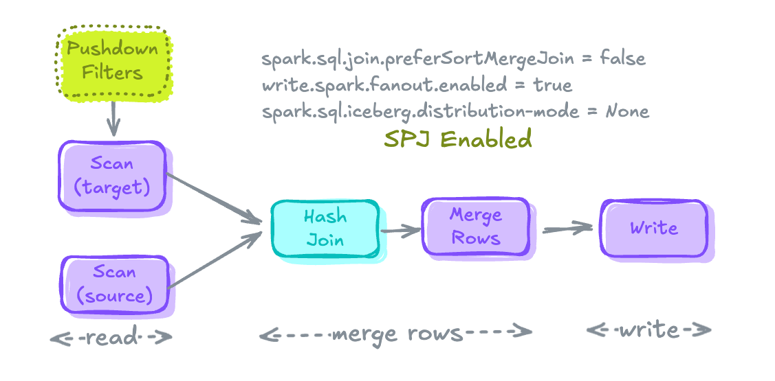
MERGE Execution Plan after StoragePartitioned Join is enabled.Let's implement all the configurations and techniques we discussed above, and rewrite the merge statements.
Optimized Merge
Let's assume in the example above that the organization introduced a new business_vertical for Data Engineers, a few of the employees moved to this vertical, and the organization hired new Data Engineers.
# Updating some employees departments after setting some configs for optimization
updated_records = spark.range(28000, 35001)\
                .withColumn("year", lit(2025))\
                .withColumn("business_vertical", lit("DataEngineering"))

updated_records.coalesce(1).writeTo(STG_TBL).overwritePartitions()
Updated data for business_vertical
Setting all the required configurations
# To avoid sort due to Sort Merge Join by prefering Hash Join if possible.
spark.conf.set('spark.sql.join.preferSortMergeJoin', 'false')

# To avoid Shuffle before writing into table.
spark.conf.set("spark.sql.iceberg.distribution-mode", "None")

# Enabling SPJ
spark.conf.set('spark.sql.sources.v2.bucketing.enabled','true')
spark.conf.set('spark.sql.sources.v2.bucketing.pushPartValues.enabled','true')
spark.conf.set('spark.sql.iceberg.planning.preserve-data-grouping','true')
spark.conf.set('spark.sql.requireAllClusterKeysForCoPartition','false')
spark.conf.set('spark.sql.sources.v2.bucketing.partiallyClusteredDistribution.enabled','true')
Setting configurations
# To avoid Pre-Sorting before writing into table
spark.sql(f"""ALTER TABLE {TGT_TBL} SET TBLPROPERTIES (
    'write.spark.fanout.enabled'='true'
)""")
Enabling fanout writers for the TARGET TABLE
Rewriting Merge Statement
Let's rewrite the MERGE statement to include:
- filter to be pushed down
year = 2025 - adding partition column
yearin join for SPJ
spark.sql(f"""
MERGE INTO {TGT_TBL} as tgt
USING (SELECT *, False as is_updated from {STG_TBL}) as src
ON tgt.id = src.id AND tgt.year = src.year AND tgt.year = 2025
WHEN MATCHED AND
    tgt.business_vertical <> src.business_vertical
    THEN
    UPDATE SET tgt.is_updated = True, tgt.business_vertical = src.business_vertical
WHEN NOT MATCHED THEN
    INSERT *
""")
Updated MERGE Statement to include filter and partition column in Join.
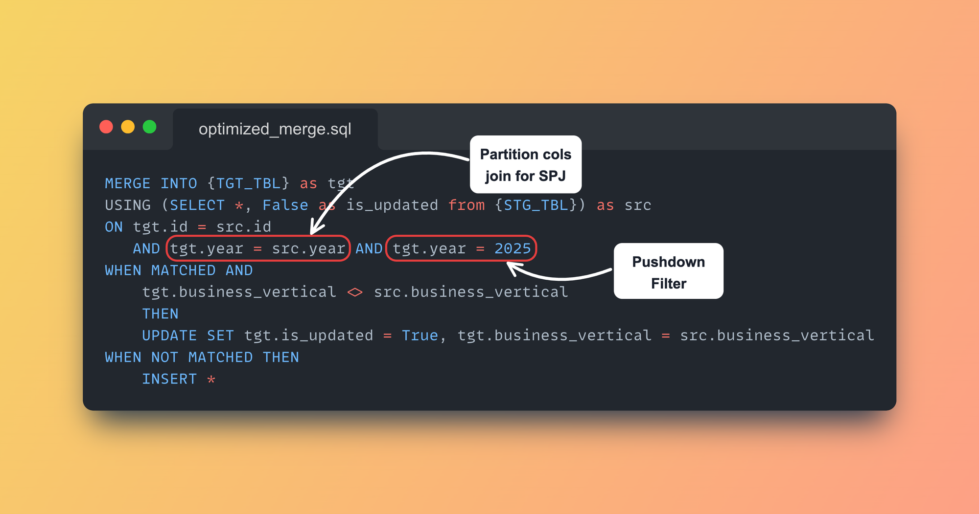
MERGE statementFinal Results
Let's look into the Spark Physical Plan for the Optimized MERGE Statement.
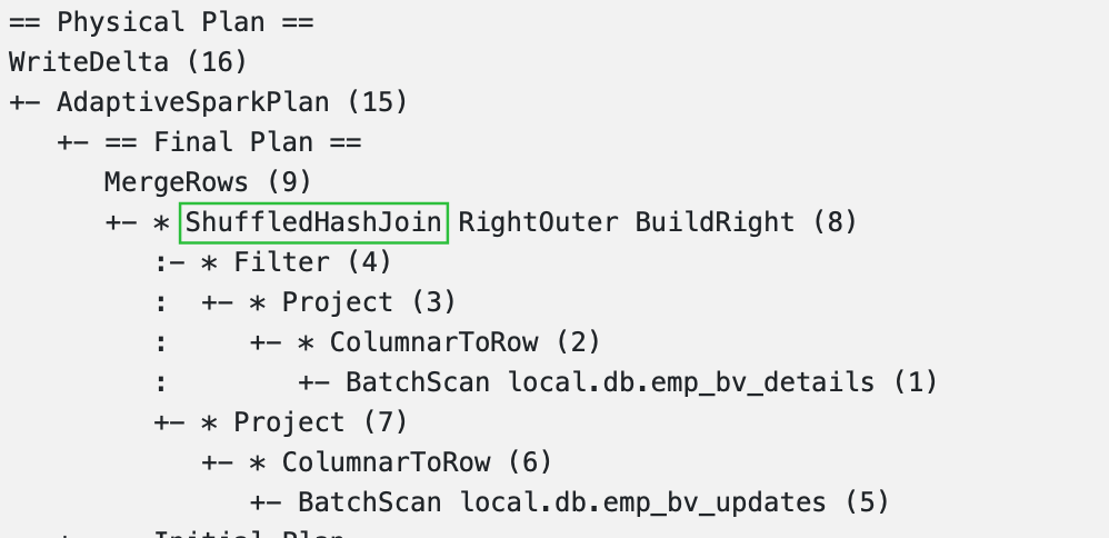
MERGE statement Physical Execution Plan- All the Expensive operations like
ExchangeandSortare not present in the plan anymore! - Sort Merge Join is converted to Shuffle Hash Join without Shuffle (thanks to SPJ).
On taking a look at the Scan Filters:
- Filters added in
ONclause are Pushed down too.
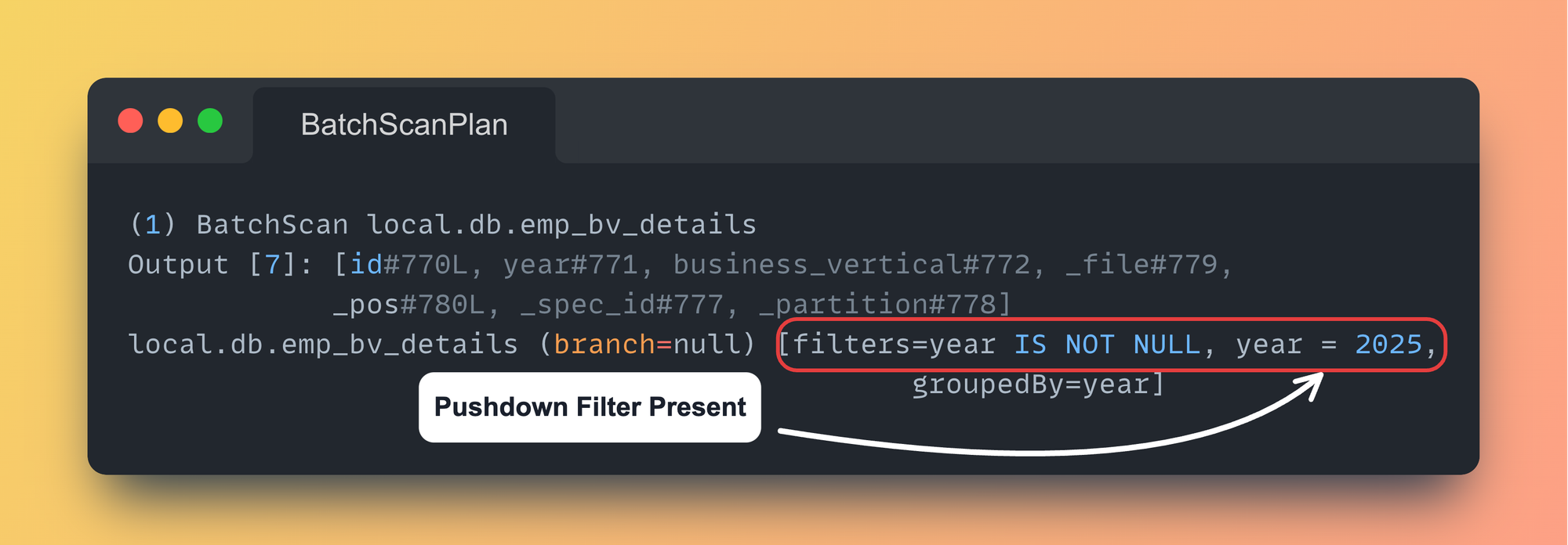
ON clause are Pushed down
TenorIf you are wondering, what happens Shuffle Hash Map Join is not possible, here's how the MERGE Execution Plan will look like:
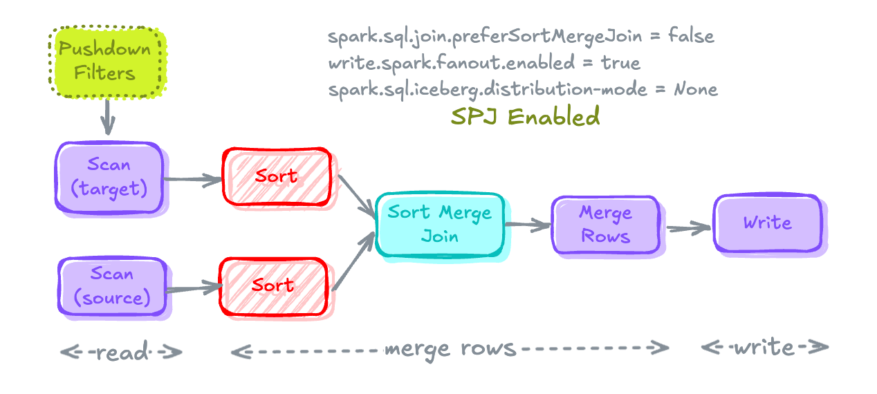
MERGE Execution Plan when Shuffle Hash Join is not possibleSort Merge Join will be there with Sort but without any Exchange.
That's it for this one! 🚀
If you have followed until here, I hope you now know:
- Expensive parts in MERGE Execution Plan.
- How to write filter conditions in MERGE Statement for it to be pushed down.
- How to enable SPJ to get rid of Shuffles while joining.
- Most importantly, you know how to optimize different parts of MERGE Execution Plan without any guess work.
Got any questions? Put it in the comments.


Member discussion